We use RMSE (Root Mean Squared Error) for evaluating the performance of a prediction model with continuous outcome. However, RMSE is not used commonly for categorical outcomes. Instead, we use a few other metrics are driven from the confusion matrix, which is introduced in the Naive Bayes handouts. Therefore, the first step of discussing the prediction power of a statistical model with a categorical outcome is forming a confusion matrix.
7.1 Confusion matrix and Miss-Classification
“Ethnicity, Insurgency, and Civil War” by Fearn and Laitin (2003) published in American Political Science Review is one the most cited studies in conflict literature. We will use this data for this session.
# It seems there is a mistake in data entry. We need to fix it:Data$onset[Data$onset>1] <-1table(Data$onset)
   0    1
6221  106
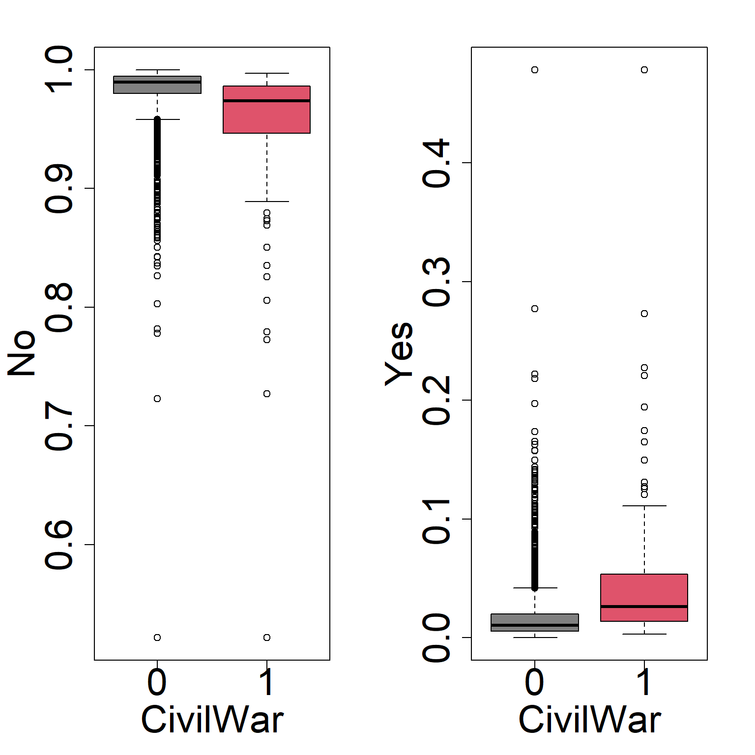
Data$onset=factor(Data$onset)library(glmnet)fm_binomial=glm(onset~warL+gdpenL+populationL+mountainous+contiguous+oil+newStata+instability+ polityL+ELF+RelELF, data = Data, family ="binomial")fm_binomial$fitted.values[1:10]
In the above example, we first estimated the probability of civil war onset, and the used a threshold, i.e.\(.5\), to categorize the predicted outcomes to zero, i.e. no civil, and 1, i.e. civil war. Indeed, in classification problems, we often estimate the probability of each category, then we pick a threshold to find the predicted categorical outcome.
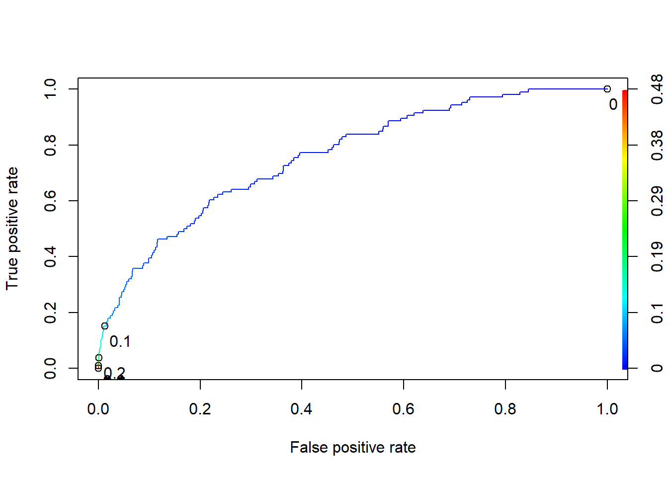
missClass=(sum(ctab)-sum(diag(ctab)))/sum(ctab)perCW=ctab[2,2]/sum(ctab[,2])cat("Missclassification and Civil War classification rate using Logit model are",round(missClass,2),"% and ",round(perCW,2),"%, respectively \n")
Missclassification and Civil War classification rate using Logit model are 0.03 % and 0.17 %, respectively
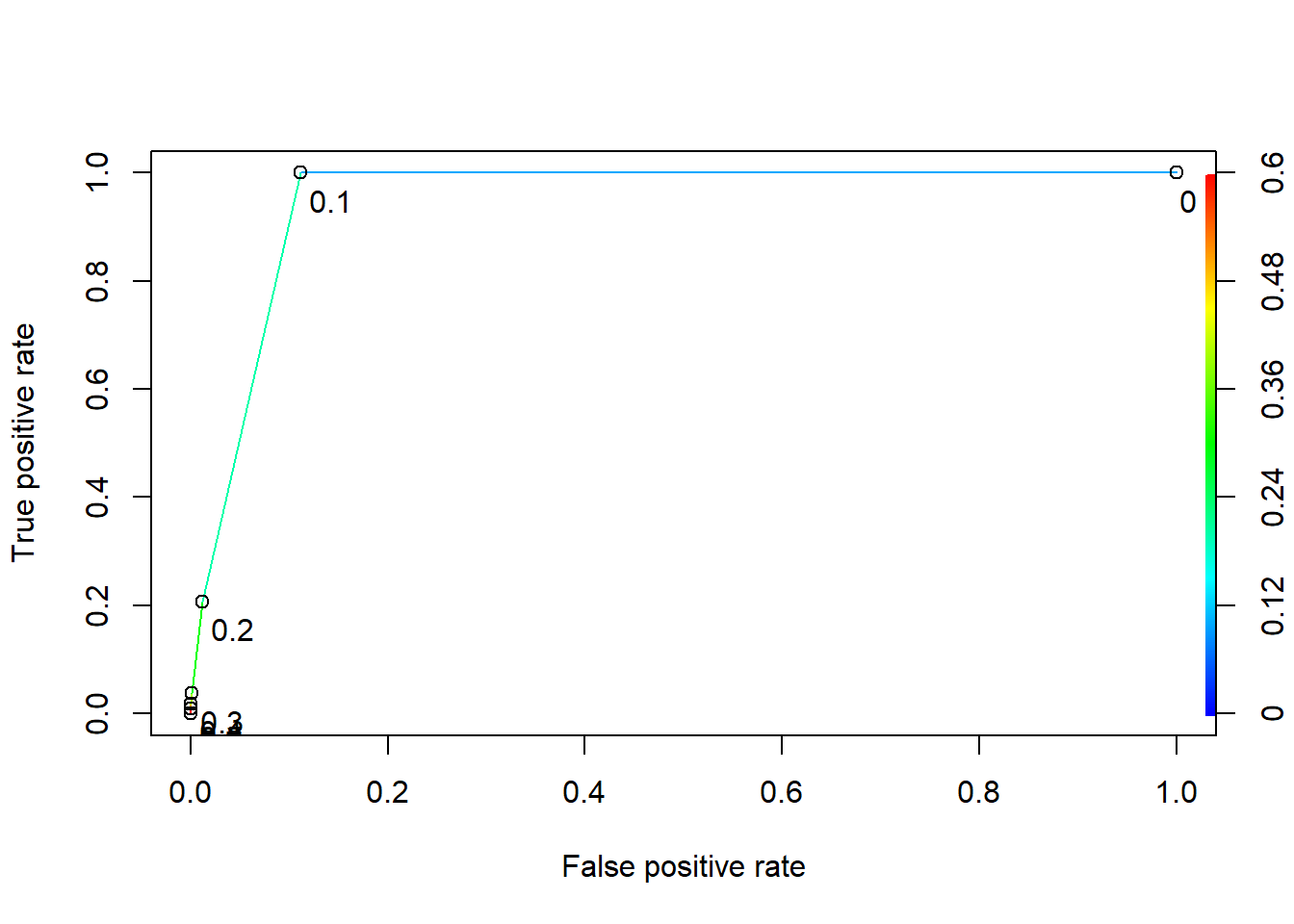
missClass=(sum(ctab)-sum(diag(ctab)))/sum(ctab)perCW=ctab[2,2]/sum(ctab[,2])cat("Missclassification and Civil War classification rate using KNN model are",round(missClass,2),"% and ",round(perCW,2),"%, respectively \n")
Missclassification and Civil War classification rate using KNN model are 0.03 % and 0.23 %, respectively
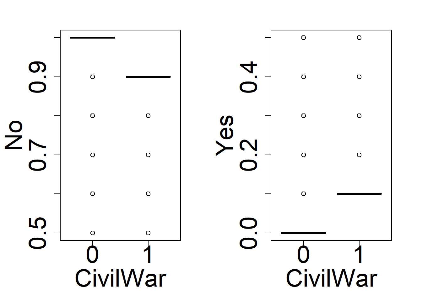
These plots presents an important issue about the quantitative models of Civil War onset. Similar to Fearon and Laitin (2003), these models are good in predicting peace, but not civil war/conflict onset!
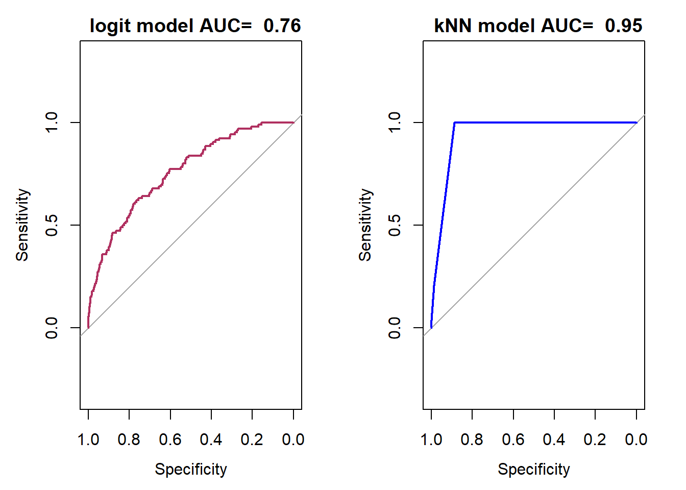
7.2 Lift, ROC, and AUC
Below graph shows the different terms that are usually used for labeling different elements of a confusion matrix. Most of the classification measures are defined using these terms/labels.
Confusion matrix
7.2.1 Lift Curve
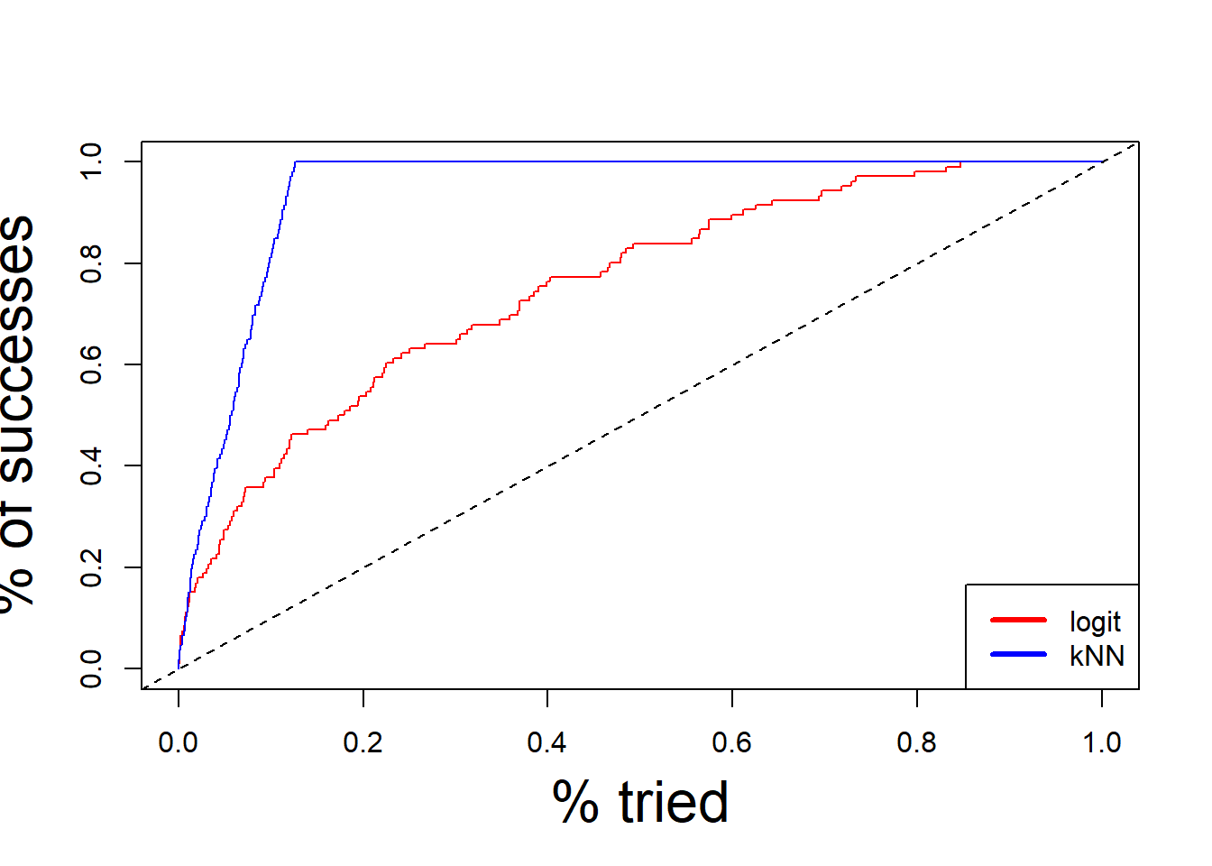
The lift curve is one of the commonly used measures of model classification performance. This measure shows how much model, that is \(\hat{p}=P(Y=1|x)\), is successful in capturing correct outcome, \(Y\).
To plot this curve, we first sort the fitting data based on \(\hat{p}\). In other words, we expect that the \(\hat{p}\) with the largest value be the one most likely to predict the correct realization of the outcome, i.e. True Positive. Then, we plot the percent observations taken vs the cumulative number of
library(devtools)source_url('https://raw.githubusercontent.com/babakrezaee/DataWrangling/master/Functions/lfitPlot_fun.R')olift =liftf(Data$onset,fm_binomial$fitted.values,dopl=FALSE)olift2 =liftf(Data$onset,fm_knn$prob[,2] ,dopl=FALSE)ii = (1:length(olift))/length(olift)plot(ii,olift,type='n',lwd=2,xlab='% tried',ylab='% of successes',cex.lab=2)lines(ii,olift,col='red')lines(ii,olift2,col='blue')abline(0,1,lty=2)legend('bottomright',legend=c('logit','kNN'),col=c('red','blue'),lwd=3)