install.packages(c("tm", "SnowballC", "caret", "e1071", "ggplot2", "pROC"))6 Evaluating AI Systems
Week 6, 7 October
Week 5 ended owing you an answer. A language model had classified a corpus of NATO tweets, the output had the right shape, and nothing in that session could establish whether any of it was correct, because those tweets carried no labels. Since then the same exercise has been run on material that does carry labels: the 181 tweets of the Week 4 test set, hand-coded by a human reading each one, given to a language model that was shown no labeled examples at all.
It agreed with the human coder on 95 percent of them. The Naive Bayes classifier of Week 4, trained on 724 hand-coded tweets, manages roughly 90 percent on the same cases. If those two numbers are the whole story, then Week 4 was a waste of an afternoon, and the sensible advice to anybody studying political text is to write a paragraph of English and stop there.
Both numbers are accurate. However, the conclusion does not follow from them, and the gap between what these two figures measure and what they are commonly taken to show is the subject of this session.
Two reasons are developed below, and they operate at different levels. The first concerns what an accuracy figure is a statement about, which turns out to be agreement with one coder’s application of one codebook rather than correspondence with the world. The second is more specific and, for anybody intending to use these labels in a project, considerably more alarming: labels that are 95 percent correct do not yield estimates that are 95 percent correct, and the error that survives is not noise but bias.
6.1 Part I. What accuracy hides
6.1.1 The classifier, rebuilt
Everything in this part runs on the Week 4 pipeline, compressed and otherwise unchanged. Nothing in the chunk below is new, and the commentary on any line of it is in last week but one.
library(tm)
library(SnowballC)
library(caret)
library(ggplot2)

url4 <- paste0("https://raw.githubusercontent.com/babakrezaee/",
               "AppliedAI-PoliSci/refs/heads/main/data/",
               "trump_immigration_2019.csv")

tweets <- read.csv(url4, stringsAsFactors = FALSE,
                   colClasses = c(id = "character"))
tweets$label <- factor(tweets$label, levels = c("other", "immigration"))

corpus <- VCorpus(VectorSource(tweets$text))

replace_with_space <- content_transformer(function(x, pattern) {
  gsub(pattern, " ", x)
})

clean <- tm_map(corpus, content_transformer(tolower))
clean <- tm_map(clean, replace_with_space, "http[s]?://\\S*")
clean <- tm_map(clean, replace_with_space, "@\\S+")
clean <- tm_map(clean, replace_with_space, "[^a-z ]")
clean <- tm_map(clean, removeWords, stopwords("english"))
clean <- tm_map(clean, stemDocument)
clean <- tm_map(clean, stripWhitespace)

dtm <- DocumentTermMatrix(clean)

train_id <- 1:floor(0.8 * nrow(tweets))

freq_words <- findFreqTerms(dtm[train_id, ], 5)

counts_train <- as.matrix(dtm[train_id, freq_words])
counts_test  <- as.matrix(dtm[-train_id, freq_words])

y_train <- tweets$label[train_id]
y_test  <- tweets$label[-train_id]

total_immigration <- colSums(counts_train[y_train == "immigration", ])
total_other       <- colSums(counts_train[y_train == "other", ])

p_immigration <- (total_immigration + 1) / sum(total_immigration + 1)
p_other       <- (total_other + 1) / sum(total_other + 1)

# The two scores, exactly as in Week 4
score_immigration <- as.vector(counts_test %*% log(p_immigration)) +
  log(mean(y_train == "immigration"))

score_other <- as.vector(counts_test %*% log(p_other)) +
  log(mean(y_train == "other"))

# Week 4 classified by asking which score was larger. The same comparison,
# written as a probability that the tweet is about immigration:
prob <- 1 / (1 + exp(-(score_immigration - score_other)))

nb_pred <- factor(ifelse(prob > 0.5, "immigration", "other"),
                  levels = c("other", "immigration"))
One line there is new, and the whole of this part depends on it.
Week 4 computed score_immigration and score_other and classified a tweet by asking which was larger. Those scores are sums of logarithms, so their units mean nothing outside the model and neither number can be interpreted on its own. The line that follows them converts the comparison into something that can be interpreted: \(P(\text{immigration} \mid \text{tweet})\), the probability the classifier assigns to a tweet being about immigration. The transformation is the logistic one, familiar from logistic regression, and it is monotone, so it changes no tweet’s position relative to any other.
The classifier’s default is to flag a tweet when that probability exceeds 0.5, which is simply the rule that a tweet goes to whichever class the model thinks more likely. Asking whether the probability exceeds 0.5 and asking whether score_immigration exceeds score_other are the same question in two notations. That cut point, rather than anything in the classifier itself, is what we are about to interrogate.
6.1.2 Precision and recall, at last
Twice now, in the Week 2 and Week 4 assignments, two numbers have been deferred with a promise that they belong here. Both describe the same confusion matrix from different directions, and both are computed with respect to a positive class that the researcher nominates.
cm <- confusionMatrix(nb_pred, y_test, positive = "immigration")

cm$table
Reference
Prediction other immigration
other 82 5
immigration 12 82round(cm$byClass[c("Precision", "Recall", "F1")], 3)Precision Recall F1
0.872 0.943 0.906 Write the four cells of that table as TP, FP, FN, and TN, where positive means immigration, and the quantities are these:
\[ \text{Recall} = \text{Sensitivity} = \frac{TP}{TP + FN} \qquad \text{Specificity} = \frac{TN}{TN + FP} \]
\[ \text{Precision} = \frac{TP}{TP + FP} \qquad F_1 = 2 \cdot \frac{\text{Recall} \times \text{Precision}}{\text{Recall} + \text{Precision}} \]
Read the denominators, because that is where the difference lives. Recall, also called sensitivity or the true positive rate, divides by everything that genuinely is immigration, so it answers a question about the cases that really are positive: of the tweets that concern immigration, what proportion did the classifier find? Precision, which caret also reports as positive predictive value, divides by everything the classifier flagged, so it answers a question about the model’s claims: of the tweets it called immigration, what proportion really were? The first is a statement about coverage, the second about trustworthiness, and a classifier can be excellent at one while being poor at the other.
Specificity is recall’s mirror image on the other class, dividing by everything that genuinely is not immigration, and it matters most when the negative class is the one you care about protecting. \(F_1\) is the harmonic mean of precision and recall, which is a way of refusing to let a model look good by sacrificing one of them entirely.
caret will report the pair you ask for, and the mode argument is worth knowing:
confusionMatrix(nb_pred, y_test, positive = "immigration",
                mode = "prec_recall")$byClass[c("Precision", "Recall", "F1")]
Precision Recall F1
0.8723404 0.9425287 0.9060773 confusionMatrix(nb_pred, y_test, positive = "immigration",
mode = "sens_spec")$byClass[c("Sensitivity", "Specificity")]Sensitivity Specificity
0.9425287 0.8723404 Neither, however, is a property the classifier possesses on its own: both are properties of the classifier taken together with a decision about where the line is drawn, and the next section makes that dependence visible.
6.1.3 The threshold is a choice, not a finding
Flagging a tweet when the probability passes 0.5 is a convention rather than a result. Any other cut point produces a different classifier from the same fitted model, and nothing in the data says that one half is the right place to stand.
cuts <- seq(0.1, 0.9, by = 0.1)

sweep_out <- data.frame()

for (cc in cuts) {
  pred_c <- factor(ifelse(prob > cc, "immigration", "other"),
                   levels = c("other", "immigration"))
  tp <- sum(pred_c == "immigration" & y_test == "immigration")
  fp <- sum(pred_c == "immigration" & y_test == "other")
  fn <- sum(pred_c == "other" & y_test == "immigration")
  tn <- sum(pred_c == "other" & y_test == "other")
  sweep_out <- rbind(sweep_out,
                     data.frame(threshold = cc,
                                flagged   = tp + fp,
                                precision = tp / (tp + fp),
                                recall    = tp / (tp + fn),
                                accuracy  = (tp + tn) / length(y_test)))
}

sweep_out$default <- sweep_out$threshold == 0.5

round(sweep_out[, 1:5], 3)
threshold flagged precision recall accuracy
1 0.1 106 0.802 0.977 0.873
2 0.2 100 0.840 0.966 0.895
3 0.3 99 0.848 0.966 0.901
4 0.4 96 0.865 0.954 0.906
5 0.5 94 0.872 0.943 0.906
6 0.6 91 0.901 0.943 0.923
7 0.7 90 0.900 0.931 0.917
8 0.8 86 0.907 0.897 0.906
9 0.9 81 0.914 0.851 0.890Read that table one row at a time, because each row is a complete confusion matrix compressed into three numbers. At a threshold of 0.1 the classifier flags a tweet on the slightest suspicion, so it finds nearly every immigration tweet and buys that coverage with false alarms. At 0.9 it flags only what it is nearly certain about, and the tweets it flags are nearly all correct, while a good many genuine ones are let through. The row marked 0.5 is the default, and it is one row among nine rather than the answer.
ggplot(sweep_out, aes(recall, precision)) +
  geom_path(colour = "steelblue", linewidth = 1) +
  geom_point(colour = "grey25", size = 1.9) +
  geom_text(aes(label = threshold), size = 3.1, colour = "grey25",
            hjust = -0.35, vjust = -0.5) +
  geom_point(data = sweep_out[sweep_out$default, ],
             colour = "maroon", size = 3.4) +
  geom_text(data = sweep_out[sweep_out$default, ],
            label = "default, p = 0.5", colour = "maroon",
            size = 3.3, hjust = 1.15, vjust = 1.8) +
  expand_limits(x = max(sweep_out$recall) + 0.04) +
  labs(x = "recall", y = "precision",
       title = "Every point is the same classifier, cut in a different place",
       subtitle = "Labels are the probability threshold for flagging a tweet")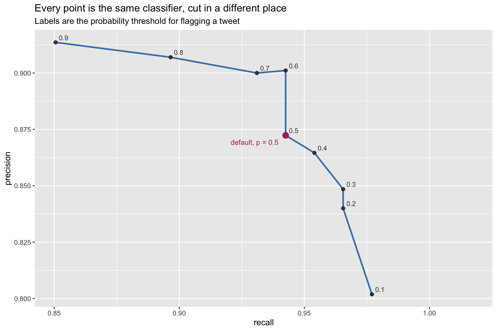
The curve falls from left to right, which is the trade-off drawn rather than described, and the labels say what it costs to move along it. There is nothing special about the maroon point. It is simply where a convention happens to put us, and its neighbors show what a different convention would have bought.
6.1.4 Why there is a trade-off at all
The curve shows that gaining one quantity costs the other, and it is worth knowing why that is inevitable rather than a quirk of this classifier.
The two measures divide by different things, and only one denominator is fixed.
Recall divides by the tweets that genuinely are about immigration. In our test set that is 87 tweets, and it stays 87 no matter what the classifier does. Precision divides by the tweets the classifier flagged, and that number is entirely under its control. Lower the threshold and it flags more, so it catches more of the real ones and recall rises. However, the extra tweets it picks up are the ones it was least sure about, so more of them are wrong, and precision falls.
Put plainly: precision is for when you need to be sure, recall is for better safe than sorry.
A spam filter is the clearest case, because almost everyone has an intuition about it already. Think about which mistake you would rather it made. A spam message reaching your inbox is a nuisance, and you delete it in a second. A real message sent to the junk folder, a job offer or an exam result, may never be seen at all. The costs are wildly unequal, so a spam filter is built for precision: when it says spam, it had better be right, and it will let some spam through to stay that way.
Now change the application and the answer flips. A screening test for a serious disease is built for recall. Missing a case is the expensive mistake, while a false alarm costs a second test and some worry, so the sensible design catches everything that might be a case and sorts out the false alarms later. Same mathematics, opposite setting.
Our classifier sits closer to the spam filter than to the screening test, which is why the default threshold of 0.5 is not obviously the right one for every purpose.
6.1.5 Try it yourself
Drag the threshold and watch the four cells move. Everything below is computed from the same 181 test tweets as the table above, and the table is laid out exactly as caret lays it out: predictions down the side, the truth across the top under the heading Reference.
Drag it to the far left and the classifier becomes paranoid, flagging nearly everything and missing almost nothing, at the cost of a great many false alarms. Drag it to the far right and it becomes cautious, flagging only what it is nearly certain of, and quietly letting real immigration tweets through. The dot never leaves the curve, because the curve is every threshold at once.
Which point on that curve is the right one is not a question the data can answer. If the labels are going to be counted, for instance to estimate what share of a year’s output concerned immigration, then false alarms inflate the count directly and precision is the quantity to protect. If the labels are going to retrieve a set of documents for a person to read, missing cases is the costly error and recall matters more, since a false alarm costs only reading time. The choice is made by the purpose, and reporting the accuracy without reporting the purpose conceals it.
6.1.6 ROC and AUC, the same sweep in the standard form
The table above is a threshold sweep, and there is a conventional way of drawing one that you will meet in every applied paper. The ROC curve plots sensitivity against one minus specificity, that is, the true positive rate against the false positive rate, as the threshold moves from one to zero.
library(pROC)

roc_nb <- roc(response = y_test, predictor = prob,
              levels = c("other", "immigration"), direction = "<")

auc(roc_nb)
Area under the curve: 0.9711plot(roc_nb, col = "steelblue", lwd = 2,
main = paste("Naive Bayes, AUC =", round(auc(roc_nb), 3)))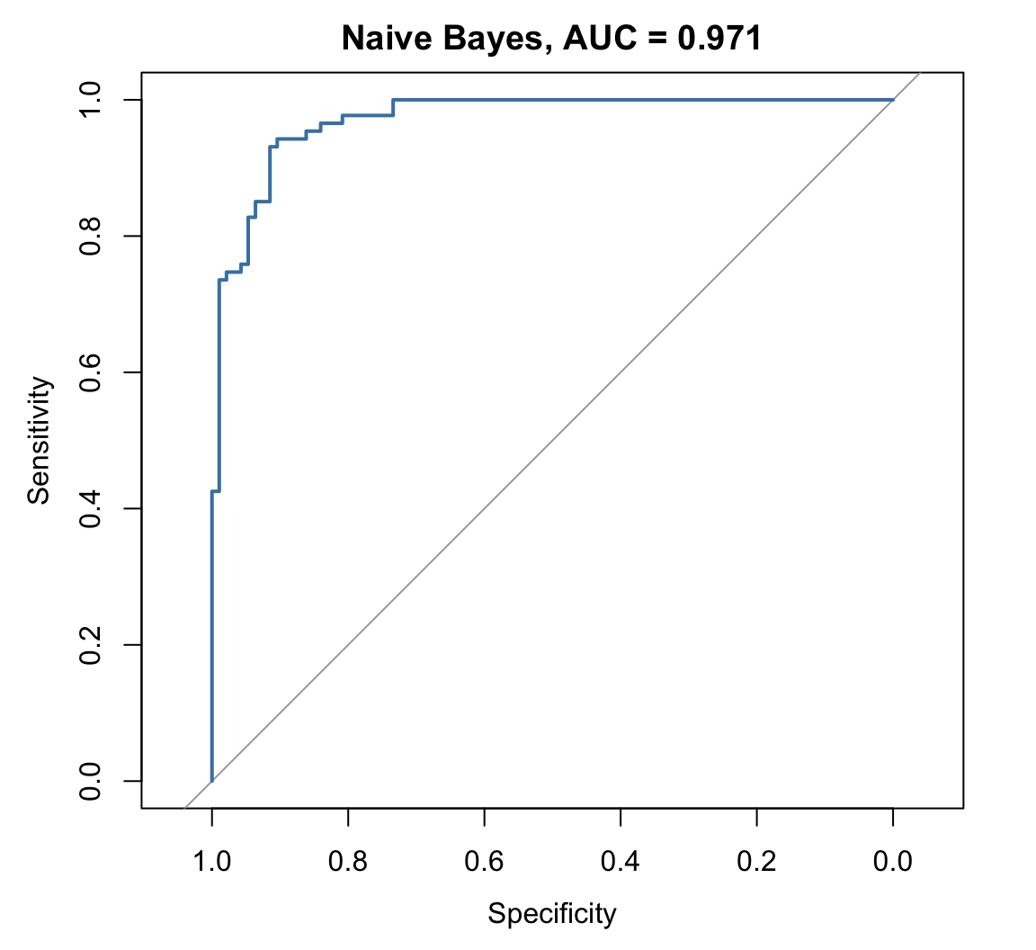
The diagonal is what a coin would achieve, since a model with no information gains a true positive for every false positive it accepts. A curve bending toward the top left is doing better than that, and the AUC, the area under the curve, compresses the whole picture into one number.
That number has a clean interpretation worth remembering, because it is not an accuracy. Take one immigration tweet and one other tweet at random. The AUC is the probability that the classifier gives the immigration one the higher score. It is therefore a statement about ranking rather than about labeling, and it does not depend on the threshold at all.
That independence is the attraction and also the trap. A model can have an excellent AUC and be useless at the threshold you actually deploy, because AUC averages over thresholds you would never choose. Report it to describe how well a model orders documents, and report precision and recall at your chosen cut point to describe what it will do in practice. Reporting only the AUC is a way of not saying what the system will actually do.
Note
There is a second curve of the same kind, the precision-recall curve, which is what we drew above. On a balanced problem the two tell much the same story. When the positive class is rare, as with civil war onset in Week 3, the ROC curve flatters a model badly, because a large number of true negatives makes the false positive rate look small however many false alarms there are. For rare outcomes, prefer the precision-recall curve.
Note
Calibration is a third property, distinct from both of these: whether a model that says seventy percent is right about seventy percent of the time. It is the central question for anything used as an early warning system, so it belongs with next week’s material on crisis management rather than here.
That is the apparatus: precision and recall, a threshold that is a decision rather than a discovery, and a curve showing what each decision costs. It was built on a classifier we fitted ourselves, which is why every part of it could be inspected.
Part II turns the same apparatus on something we did not build and cannot open.
6.2 Part II. Validating a language model
Week 5 ended with an admission. A language model had classified a corpus, the output had the right shape, and nothing in that session established whether any of it was correct, because the NATO tweets carried no labels to check against. The instrument required was the one Week 4 built, and it is applied here.
Two systems are now in play, so the naming below is fixed and used consistently. The classifier is the Naive Bayes model of Week 4, trained on 724 hand-coded tweets. The model, or the language model, is the one from last week, which was trained on nothing of ours and told what to do in a paragraph of English.
url6 <- paste0("https://raw.githubusercontent.com/babakrezaee/",
               "AppliedAI-PoliSci/refs/heads/main/data/",
               "llm_labels_w6.csv")

llm <- read.csv(url6, stringsAsFactors = FALSE,
                colClasses = c(id = "character"))

str(llm)
'data.frame': 181 obs. of 7 variables:
$ id : chr "1124672389416144905" "1120715879640174592" "1106205023548133376" "1173803449202249728" ...
$ date : chr "2019-05-04 21:49" "2019-04-23 23:47" "2019-03-14 22:46" "2019-09-17 11:38" ...
$ text : chr "Very good call yesterday with President Putin of Russia. Tremendous potential for a good/great relationship wit"| __truncated__ "Great interview by Jared. Nice to have extraordinarily smart people serving our Country! https://t.co/d6Tgrn4Tzn" "A vote for today’s resolution by Republican Senators is a vote for Nancy Pelosi, Crime, and the Open Border Democrats!" "Beautiful evening in New Mexico with Great American Patriots! https://t.co/S8eDG3dAq0" ...
$ human : chr "other" "other" "immigration" "other" ...
$ llm_main : chr "other" "other" "immigration" "other" ...
$ llm_reword: chr "other" "other" "immigration" "other" ...
$ llm_model2: chr "other" "other" "immigration" "other" ...6.2.1 What is in the file, and where it came from
The file carries four labels for every tweet, and the rest of this part is built on the differences between them, so it is worth being precise about what each one is.
| Column | What produced it |
|---|---|
human |
The Week 4 hand coding, one person working from a written codebook |
llm_main |
A language model, given the prompt below, called prompt A |
llm_reword |
The same model on the same tweets, given a differently worded prompt saying the same thing, called prompt B |
llm_model2 |
A different model from the same provider, given prompt A again |
So two things vary, and only one at a time. Comparing llm_main against llm_reword holds the model fixed and changes the wording. Comparing llm_main against llm_model2 holds the wording fixed and changes the model. The exact model names and the date of the run are recorded in data/llm_labels_w6_README.md, since a measurement of this kind is meaningless without them.
A word on what “a different model” means here, because the vocabulary is looser than it looks. Both models come from the same provider and the same family, trained in the same way on much the same material, and they differ in scale: the number of parameters and the quantity of computation behind each answer. Providers rarely publish those numbers, so the practical signals available to you are the price per token and whatever tier name the provider has given it. The one used for llm_model2 is the more expensive of the two. That matters for how much the comparison is worth, and the point is taken up at the end of this part: two models from one company are not two independent opinions.
Both prompts were written to do the same job, and neither is a straw man.
Prompt A, which produced llm_main and llm_model2:
You are coding tweets for a political science project.
Decide whether immigration is a main subject of the tweet. This includes the southern border, the border wall, illegal immigration, deportation, ICE, sanctuary cities, asylum, visas, and DACA.
If immigration is mentioned only in passing within a longer list of topics, code it as other.
Prompt B, which produced llm_reword:
Classify each tweet by topic.
Answer immigration if the tweet concerns immigration or border policy in any substantial way. Answer other for everything else.
Read them side by side before going on, because the comparison later depends on your judgment that these are two reasonable attempts at one instruction rather than a good prompt and a bad one. Prompt A is longer, gives examples, and states the rule about passing mentions. Prompt B is shorter and leaves “substantial” to the model. Either is the sort of thing a researcher writes first, and neither contains an error.
The script that produced the file is in the repository at R/w6_generate_llm_labels.R, and the provenance, including what is and is not reproducible about it, is in data/llm_labels_w6_README.md. Read both before the session. The session concerns evaluation, and a measurement whose origin is undocumented cannot be evaluated at all.
6.2.2 Three label sources, one set of tweets
human <- factor(llm$human, levels = c("other", "immigration"))
llm_main <- factor(llm$llm_main, levels = c("other", "immigration"))

confusionMatrix(nb_pred, human, positive = "immigration")$table
Reference
Prediction other immigration
other 82 5
immigration 12 82confusionMatrix(llm_main, human, positive = "immigration")$table Reference
Prediction other immigration
other 87 2
immigration 7 85round(rbind(
naive_bayes = confusionMatrix(nb_pred, human,
positive = "immigration")$byClass[c("Precision", "Recall")],
llm = confusionMatrix(llm_main, human,
positive = "immigration")$byClass[c("Precision", "Recall")]
), 3) Precision Recall
naive_bayes 0.872 0.943
llm 0.924 0.977The language model outperforms the classifier, and it does so having been shown no training data at all. The result is real and should be taken seriously, since it is close to what the published literature reports.
However, the shape of the model’s errors tells us more than the headline figure does. Recall is much higher than precision, which means the model rarely misses an immigration tweet and fairly regularly flags one the coder did not. Rather than theorize about why, we can read the mistakes.
wrong <- llm[llm$human != llm$llm_main, c("text", "human", "llm_main")]

nrow(wrong)
[1] 9false_alarms <- wrong[wrong$human == "other", ]
for (i in 1:nrow(false_alarms)) {
cat("-", substr(false_alarms$text[i], 1, 190), "\n\n")
}- ....Kevin is strong on Securing the Border, #USMCA, protecting our #2A, and Loves our Vets and Military. Kevin is a true friend, and has my Complete and Total Endorsement!
- MISSISSIPPI! There is a VERY important election for Governor on November 5th. I need you to get out and VOTE for our Great Republican nominee, @TateReeves. Tate is Strong on Crime, tough on
- Senator Cindy Hyde-Smith is doing a GREAT JOB for the people of Mississippi and fully supports our #MAGA Agenda. Cindy is tough on Crime, Strong on the Border and Illegal Immigration....
- I will be signing our 738 Billion Dollar Defense Spending Bill today. It will include 12 weeks Paid Parental Leave, gives our troops a raise, importantly creates the SPACE FORCE, SOUTHERN B
- ..that this Administration has done. They don’t talk about the great economy, the big tax and regulation cuts, the rebuilding of the Military, “Choice” at our VA, our Vets, Judges and Suprem
- Looking forward to being in the North Carolina tomorrow night. We’re having a BIG RALLY for a great guy, Dan Bishop. Strong on Crime, Borders, your Military and our Vets, we need Dan Bishop
- I will be interviewed by Jeanine Pirro at 9:00 P.M. on @FoxNews. Watch @JesseBWatters before and @greggutfeld after. All terrific people. I am in the White House waiting for Cryin’ Chuck and Six of these seven are the same kind of tweet. They are campaign endorsements and lists of accomplishments, in which the border appears as one item in a series: strong on crime, strong on the border, protects the Second Amendment, loves our veterans. The defense spending bill tweet is the purest case, since “SOUTHERN BORDER WALL FUNDING” sits in a list alongside parental leave, a troop pay raise, the Space Force, and the smoking age.
Now recall where those tweets got their labels. The Week 4 codebook has a rule for exactly this situation: a passing mention inside a longer list is coded other. A second rule covers endorsement boilerplate, on the grounds that the border in such a tweet occupies one slot in a formula rather than serving as its subject. Those rules were written by one person, in an afternoon, to resolve cases the original scheme had not anticipated.
So the model is not misreading English. It is reading these tweets much as you or I would, noticing that immigration is mentioned, and failing to apply a convention that a human coder invented and wrote down somewhere the model never saw. Its errors concentrate almost entirely on the cases where the codebook had to make a judgment call.
missed <- wrong[wrong$human == "immigration", ]

for (i in 1:nrow(missed)) {
  cat("-", substr(missed$text[i], 1, 190), "\n\n")
}
- So now the Obama appointed judge on the Census case (Are you a Citizen of the United States?) won’t let the Justice Department use the lawyers that it wants to use. Could this be a first?
- ....This will supersede USMCA. Likewise I am looking at an economic penalty for the 500 Billion Dollars in illegal DRUGS that are shipped and smuggled through Mexico and across our Southern The two it missed point the same way. One concerns the census citizenship question, which the codebook counts as immigration and which a reasonable person might not. The other is about drugs smuggled across the southern border, where the codebook says that drugs count only when the tweet ties them to immigrants or the border, and this tweet arguably does. Neither is a stupid mistake, and both are disagreements about a rule rather than about the tweet.
Keep this in mind for Part III, because the whole session turns on it. Our 95 percent is not a measure of how well the model understands immigration. It is a measure of how often it happens to apply the same conventions as one human coder, and the five percent where it fails is made almost entirely of the places where those conventions were contestable.
One further asymmetry between the two systems is worth drawing out, since it did not appear in the table. The classifier produced a ROC curve in Part I because it reports a probability, so a threshold can be moved through it and a whole family of classifiers obtained from one fit. The language model reports a label and nothing else. It is therefore a single point in that space rather than a curve, with one sensitivity and one specificity, and no dial to turn. Whatever trade-off between precision and recall it happens to embody was fixed by the prompt and the model, and if it over-flags, as this one does, the only instruments available are rewriting the prompt or asking the model for a probability and hoping it means something. The classifier gives you a worse result and more control over it.
6.2.3 Four ways to shake a measurement
What we have so far is one measurement, taken once, by one model, under one prompt. It agreed with the coder 95 percent of the time. Before that number can be believed, it is worth asking whether it would survive the kinds of variation that any real research project will inflict on it without meaning to.
Four questions do that, and they are arranged so that each holds more fixed than the last. The first asks whether the model’s claims survive being checked against the world. The second changes the wording of the instruction. The third changes the model. The fourth changes nothing at all. If a measurement cannot survive the fourth, the earlier three were never the problem.
6.2.4 Check one, the existence check: does the claim survive looking up?
This check applies whenever a model asserts something that could in principle be looked up. Ask it for a source, then verify that the source exists and says what the model says it says.
Nothing in the file above bears on this, since it is not a classification problem, which makes it a workshop exercise rather than a chunk here. Use something you can actually check, and Fearon and Laitin’s 2003 article serves well, since it is on the Week 3 reading list and already in your possession:
Ask the model what Fearon and Laitin found about the relationship between ethnic diversity and civil war onset, and then ask it for the page on which they report it. Open the article and look.
Then do the same with an article you know well from another course, and then with one you have only heard of. The third is the interesting case, because it is the one where you would have believed the answer.
What you are looking for is not an error of the ordinary kind. It is a reference with a plausible author, a plausible journal, a plausible year, and a page number, for an article that does not exist, or a real article that says something else. The output gives you nothing to go on, since a fabricated citation is written in exactly the same confident register as a correct one.
The point is larger than the trick. In Part II we treated the model’s labels as data, and the only reason we could trust them at all is that we had 181 human judgments to check them against. The moment a model asserts something you cannot check, you are relying on fluency as a proxy for accuracy, and these are separate properties of a text. Only one of them is visible without leaving the page.
6.2.5 Check two, prompt stability: does the answer survive a reworded prompt?
The existence check concerns what a model asserts. The remaining three concern whether a measurement holds still, and the first thing to vary is the one a researcher varies most casually: the wording of the instruction.
llm_reword <- factor(llm$llm_reword, levels = c("other", "immigration"))

table(as_written = llm_main, reworded = llm_reword)
reworded
as_written other immigration
other 82 7
immigration 0 92round(mean(llm_main == llm_reword), 3)[1] 0.961Prompt A and prompt B are both defensible, as you saw above, and the model is identical in the two runs. The only thing that changed between them is the wording of the instruction. Yet a share of the corpus is labeled differently depending on which was used, and the identity of those tweets is more instructive than their number.
moved <- llm[llm$llm_main != llm$llm_reword, ]

for (i in 1:nrow(moved)) {
  cat("-", substr(moved$text[i], 1, 170), "\n\n")
}
- ....energy independence, manufacturing resilience, illegal immigration coming down, the Wall going up, China confronted, the caliphate defeated, NAFTA renegotiated, our m
- So now the Obama appointed judge on the Census case (Are you a Citizen of the United States?) won’t let the Justice Department use the lawyers that it wants to use. Coul
- ....This will supersede USMCA. Likewise I am looking at an economic penalty for the 500 Billion Dollars in illegal DRUGS that are shipped and smuggled through Mexico and
- All necessary work has been completed to declare Mexican Cartels terrorist organizations. Statutorily we are ready to do so. However, at the request of a man who I like a
- “Poll shows Dems losing interest in Impeachment inquiry all across the board. These Polls are actually devastating to the Democrats. But the writing was on the wall. He’s
- It was a very bad week for the Democrats, with the GREAT economic numbers, The Virginia disaster and the State of the Union address. Now, with the terrible offers being m
- The White House will be hosting a very big and very important Social Media Summit today. Would I have become President without Social Media? Yes (probably)! At its conclu These are the same families of tweet as the errors above. There is the long list of accomplishments with “illegal immigration coming down” buried in it, the census citizenship question again, the drug smuggling tweet again, and a poll quotation that mentions building the wall in passing. The tweets that move when the prompt moves are the tweets that were ambiguous under the codebook in the first place.
That is reassuring and alarming in about equal measure. Reassuring, because the instability is not random: the model wavers exactly where a careful human coder had to stop and make a decision. Alarming, because those borderline cases are frequently the substantively interesting ones, and because a researcher who ran only one prompt would never learn that an eighth of the ambiguous cases could have gone the other way.
Set that share against the error rate from the previous section. The model disagrees with the human coder on about five percent of tweets, and it disagrees with itself under rewording on about four percent. The instability introduced by a reasonable change of wording is therefore nearly as large as the measured error, which means that a paper reporting the accuracy of such a classifier without reporting its sensitivity to the prompt has reported roughly half of what the reader needs.
6.2.6 Check three, inter-model reliability: does a second model agree?
Here the wording is held fixed and the model changes. Two models were used, and the difference between them matters for how much the comparison is worth.
llm_model2 <- factor(llm$llm_model2, levels = c("other", "immigration"))

table(prompt_A_model_1 = llm_main, prompt_A_model_2 = llm_model2)
prompt_A_model_2
prompt_A_model_1 other immigration
other 83 6
immigration 1 91round(mean(llm_main == llm_model2), 3)[1] 0.961That is a second model from the same company, which is a weak kind of independence. Two models built by one firm, trained in similar ways on similar text, are closer to two readings from one instrument than to two instruments. If they share an assumption about what the word “border” implies, they will agree because of it rather than despite it.
So we ran prompt A a third time, through a model from a different company. The same ellmer code does this; only the function changes, from chat_openai() to chat_anthropic(), which is the practical argument for using a package that is not tied to one provider.
url_c <- paste0("https://raw.githubusercontent.com/babakrezaee/",
                "AppliedAI-PoliSci/refs/heads/main/data/",
                "llm_claude_w6.csv")

claude <- read.csv(url_c, stringsAsFactors = FALSE,
                   colClasses = c(id = "character"))

llm_claude <- factor(claude$llm_claude, levels = c("other", "immigration"))

round(c(same_company  = mean(llm_main == llm_model2),
        other_company = mean(llm_main == llm_claude)), 3)
same_company other_company
0.961 0.950 The expectation was that agreement across companies would be clearly lower. It is lower, and by two tweets out of 181, which is nothing. We looked for the effect, did not find it at this sample size, and are reporting that rather than quietly dropping the comparison, which is the practice this session is supposed to be teaching.
A more useful question is what happens when all three agree.
unanimous <- llm_main == llm_model2 & llm_main == llm_claude

sum(unanimous)
[1] 169table(all_three_said = llm_main[unanimous], human = human[unanimous]) human
all_three_said other immigration
other 81 0
immigration 3 85The three models give the identical label on 169 of the 181 tweets. On those 169, they match the human coder 166 times. Three systems, two companies, in unanimous agreement, and still wrong three times.
Those three tweets are the point of the next section. No amount of agreement among models would have found them. The only thing that did was a person who had read the tweet.
6.2.7 Check four, intra-model reliability: does the same model agree with itself?
This is the simplest of the four, and the most unsettling. The three before it changed something: the wording, or the model. This one changes nothing at all. Run the identical prompt, on the identical model, a second time, and see whether the answers match. If check three asks whether a different model agrees, check four asks whether the same model agrees with itself.
It does not. Run twice over these 181 tweets, the model disagreed with itself on 8 of them, and the accuracy against the hand labels moved from 95.0 percent on one run to 93.9 percent on another. Nothing was altered between the runs. The question was the same, the model was the same, and the number you would have written in your paper depends on which afternoon you ran it.
Five of those eight tweets are the same ones that flip when the prompt is reworded. Counting everything that moved under any of the three perturbations, rewording, changing model, or simply asking again, the total is 12 tweets out of 181. The model is immovable on about 93 percent of the corpus and close to flipping a coin on the rest, and that unstable remainder is the same set of borderline cases the Week 4 codebook needed its tie-break rules for. The checks were not measuring three different things. They were finding the same ambiguous tweets by three different routes.
6.2.8 Why that happens, and why we could not switch it off
Week 5’s first diagram showed the model producing a probability for every possible next token, and something then choosing one. Temperature is the dial on that choice.
At a temperature of zero the model always takes the most likely token. The same question gives the same answer every time, which is dull for writing and exactly what you want for measurement. Turn the dial up and the choice becomes a draw rather than a maximum, so less likely tokens become reachable, the output is more varied, and repeated calls stop agreeing. For years the standard advice to anybody using these models as a research instrument was therefore simple: set the temperature to zero and report that you did.
That advice no longer works here, and the reason is worth understanding.
The model we are using is a reasoning model. Rather than answering immediately it first generates a chain of intermediate steps, working through the problem before committing, and only then produces the answer. That internal process was built and tuned at one particular setting of the dial. Turning the dial down would not make such a model more reliable; it would interfere with the very process the model was trained to carry out, and the provider has judged that the result would be worse rather than more repeatable. So the setting is locked.
It is locked firmly. We asked for a temperature of zero on all 181 tweets and every single call was refused, with the API replying that only the default value is supported. A setting of 0.5 is refused in the same way. The parameter exists in the R package, it is named in every methods paper on this subject, and on this model you may not use it.
Sit with the consequence rather than the inconvenience. The standard remedy for non-determinism is unavailable, not because of a limitation of the method but because a company decided that you should not have it, for reasons that are probably sound and that you are in no position to evaluate. You can still report the instability, which is what the eight tweets above do. You cannot remove it.
6.2.9 Agreement is not accuracy
Several agreement rates have now been produced, and the temptation is to read them as so many measurements of the same thing. They are not, and the distinction is the most important idea in this part.
Agreement between two prompts, between two models, between two companies, or between two runs of the same model establishes that a measurement is reproducible. It says that the number would come out much the same if somebody else ran it, which is a real property and not a trivial one. However, it says nothing whatever about whether the number is right. Models trained on overlapping corpora, with overlapping assumptions about what the word “border” implies, may agree with one another precisely because they share a bias, and their agreement is then evidence of a common error rather than of a correct answer. Check three showed exactly that, three times over.
Only the human labels speak to accuracy. Thus the comparison that matters is the first one, against human, and the reliability checks are supporting evidence rather than substitutes.
That said, the human labels are themselves a measurement rather than the truth. They were produced by one coder applying one written codebook, and the Week 4 documentation records the four rules invented to resolve cases the scheme did not anticipate. A second coder would place some tweets differently. The honest statement of the result is therefore not that the model is 95 percent accurate, but that it agrees 95 percent of the time with one person’s application of one coding scheme to 181 tweets. Every further claim rests on that sentence, and it is a good deal weaker than the number alone suggests. On the practice of treating human judgment as the benchmark, and on what that requires, see Lowe and Benoit (Lowe and Benoit 2013).
Part II has established how far the number can be trusted as a measurement of what the coder did. Part III asks a harder question: whether what the coder did is what we wanted measured, and whether the test was a test at all.
6.3 Part III. Why a good score can be the wrong number
6.3.1 What the score is a score of
Political scientists have a word for the problem this section is about, and it is one of the few places in this course where the discipline is ahead of computer science rather than behind it. Construct validity asks whether an instrument measures the concept it claims to measure, as distinct from measuring something close to it, something correlated with it, or something merely easier to count.
The number in Part II is an agreement rate against a codebook. Whether it is also a measure of the aboutness of immigration depends entirely on whether the codebook captured that concept, and that codebook was the work of a single coder resolving awkward cases as they arose. Rule one of it, which sends a tweet listing ten accomplishments with “Border” seventh into the other category, is a judgment call that a different coder could defensibly reverse. Reverse it, and the labels change, and the model’s accuracy against the new labels changes, and nothing about the model or the tweets has moved at all.
Four questions bear on any evaluation, and they are not one question asked four times. Each one can be put to our own classifier.
Does the measure cover the concept, or only part of it? Our scheme counts a tweet about the census citizenship question as immigration and a tweet endorsing a candidate who is “strong on the border” as not. A reader who thinks immigration politics is substantially about how politicians signal toughness on it would say we have measured the policy debate and discarded the political performance, which for many research questions is the half that matters.
Does it agree with an established measure of the same thing? The Comparative Agendas Project and the Manifesto Project have both coded political text for immigration content for years, using schemes refined over decades by multiple coders. Ours was the work of one person over a few hours. We never checked our labels against either, and we could have.
Does the measure behave as the concept should behave? Here we do reasonably well. The immigration share falls sharply after the first half of 2019, which is what anybody following the shutdown and then impeachment would expect, and a measure that showed no such movement would be suspect regardless of its agreement rate.
What follows from using it? Suppose this classifier were not a teaching exercise but a monitoring system, and suppose politicians learned which words triggered it. The endorsement tweets in Part II show that the border can be invoked while saying nothing about it, and a measure deployed at scale eventually changes the behavior of whoever is being measured.
An evaluation that answers only the question “how often does it agree with my labels” has addressed the first of these badly and the other three not at all.
6.3.2 When the test was not really a test
A score can also be too high for a reason that has nothing to do with the concept. It can be too high because the test was not a test.
The idea is the same one that makes an exam meaningful. An exam measures what a student knows only if the student has not seen the questions beforehand. Show them the paper during revision and they will score well, the marking will be correct, the arithmetic will be sound, and the number will mean nothing about what they would do on an exam they had not seen.
The same thing happens to models, and it has a name. Leakage is any way in which information from the test set reaches the model before it is tested. It does not require cheating or carelessness. It usually happens through a decision that looks like housekeeping.
We can produce it deliberately, in one line, and watch it work. The first route runs through the vocabulary.
Part I built the classifier’s vocabulary from the training tweets only. Here is that line again, beside the version that forgets to do so.
# What Part I did: look only at the 724 training tweets, and keep every word
# used at least 5 times among them.
length(freq_words)
[1] 651# The careless version: look at all 905 tweets, including the 181 that are
# about to be used as the test set.
freq_leaky <- findFreqTerms(dtm, 5)
length(freq_leaky)[1] 749dtm is the full matrix of 905 tweets. dtm[train_id, ] is just the 724 training rows, which is what Part I passed to findFreqTerms(). Dropping that [train_id, ] is the whole mistake, and it is one keystroke.
The careless vocabulary is larger, by around a hundred words. Those extra words are the interesting part, and setdiff() isolates them: it returns the items in the first set that are not in the second.
head(setdiff(freq_leaky, freq_words), 20) [1] "account" "addit" "address" "amaz" "appoint"
[6] "apprentic" "assist" "associ" "benefit" "biden"
[11] "bishop" "black" "bless" "brought" "captur"
[16] "center" "condit" "congression" "consider" "convers" Each of these is a word that was not frequent enough among the training tweets to qualify, and became frequent enough only once the test tweets were counted. They are in the model’s vocabulary because of documents it is about to be graded on. Every one of them is now a feature the classifier can use, and the classifier has been told something about its own exam.
The second route is easier to take, and we took it in Part I. It runs through a choice rather than through a line of code.
That threshold table reported precision, recall, and accuracy at nine cut points, all computed on the test set. Nothing is wrong with looking. The question is what happens if you then pick.
# The row of the sweep where accuracy happens to be highest.
# which.max() returns the position of the largest value in a vector.
best <- sweep_out[which.max(sweep_out$accuracy), ]

# sweep_out$default is the TRUE/FALSE column marking the 0.5 row, so this
# compares the accuracy at the default against the best available anywhere.
round(c(at_the_default = sweep_out$accuracy[sweep_out$default],
        best_on_test   = best$accuracy), 3)
at_the_default best_on_test
0.906 0.923 best$threshold[1] 0.6The best threshold is not 0.5, and it delivers a visibly higher accuracy, worth a few more tweets correct. We could report that number. It came out of real code, run on real data, with no mistake anywhere in it.
It would still be false as a statement about new tweets, because the threshold was chosen by looking at the answers. We did not estimate which cut point works; we looked up which cut point happened to work here. On the next 181 tweets it would not be the best, and the figure we reported would not be reproduced.
Notice what this episode did not include. No error message, no warning, no suspicious output, and no moment at which anybody did anything that felt wrong. Leakage does not announce itself as a bug. It announces itself as a better result. That is why it survives peer review.
6.3.3 The version you cannot check
Both examples above are repairable. Pass dtm[train_id, ], choose the threshold on data the model has not been judged on, and the problem goes away.
Now the same problem in a form where nothing can be done. Contamination is leakage into a model you did not train: the possibility that your test documents were part of the training data of the model you are testing. With a commercial language model, whose training corpus is undisclosed, the honest position is not that this did not happen. It is that you cannot know.
Our own case is not hypothetical. These are tweets by a sitting president, quoted in thousands of news articles, analysed in academic papers, and archived in at least three public GitHub repositories, including the one this corpus was built from. If any text on the internet was in that training data, this text was. The model may well have met these exact tweets before, accompanied by journalism explaining what each was about, which is considerably more than the paragraph of instruction we gave it.
This cannot be checked by us or by anyone outside the company, and it is not a reason to abandon the method. It is a reason to write the limitation down rather than report 95 percent as though it were a clean out-of-sample result.
It also unsettles the comparison in Part II. The Naive Bayes classifier saw 724 tweets and nothing else in its entire existence. The language model may have seen these tweets and the commentary about them. The contest was never as fair as the table made it look, and the fairer reading of Part II is that a system with an unknown and probably large advantage beat one with none.
6.3.4 What a benchmark number means
Published evaluations of these systems are mostly benchmark scores, and three pathologies recur often enough to be recognizable. Two of them we have already committed in this handout, which is the quickest way to understand them.
Benchmarks saturate. Once a test is widely used, systems are built and selected against it until the leading ones all score within a point or two of each other and of the ceiling, at which stage the test has stopped ranking the systems and started ranking the noise. The remedy is a harder test, so the cycle runs again, and the published scores across a few years of such cycles are not comparable with one another.
Benchmarks are gamed, though rarely by fraud. The ordinary mechanism is the one from the previous section: we swept a threshold across our test set and could have reported the best value we found. Nobody lied, no rule was broken, and the reported figure would still have described our test set rather than the world. Scale that up to an industry in which benchmark position determines funding and procurement, and the pressure runs the same way without anybody deciding that it should.
And a growing share of evaluation now uses one language model to judge the output of another, since human raters are slow and expensive. This is efficient and it is circular, for the reason Part II gave: a judge trained on much the same text as the system it grades will share its assumptions about what a good answer looks like, so agreement between them is weak evidence of quality. We saw the small version of this in check three: three models agreed unanimously on 169 tweets and were wrong on three of them, and nothing about their agreement revealed which three.
The practical conclusion is narrow, and it is the one thing from this section to carry out of the room. When a procurement document, a vendor, or a paper reports that a system is 94 percent accurate, the figure is a claim about performance on some benchmark, and the questions that matter are which one, constructed by whom, measured when, and against whose labels. None of those is a technical question, and a political scientist is as well placed to ask them as anybody.
6.4 Part IV. When the measurement feeds a regression
Everything so far has treated the labels as the end product. In a research project they almost never are. The labels become a variable, the variable enters an analysis, and the analysis produces the number that appears in the abstract.
Take a question we can actually ask of these 181 tweets. Immigration dominated the first part of 2019, through the shutdown over wall funding and the national emergency declaration, and receded later in the year as impeachment took over. How much larger was the immigration share in the first half of the year than in the second?
Split the test tweets by half of the year, compute the immigration share in each half, and take the difference. Do it three times, once with each set of labels. The hand labels put the gap at roughly 36 percentage points. The model’s labels put it at roughly 30, and the reworded prompt at roughly 27. A classifier that is right 95 percent of the time has understated a substantively central quantity by something between a sixth and a quarter.
The mechanism is general, and worth following through once. The model over-flags, as Part II established, so it adds spurious immigration tweets in both halves of the year. In the second half, where genuine immigration tweets are scarce, those additions are a much larger share of the total. The second-half figure is therefore inflated more than the first-half figure, the gap between them narrows, and the result is pulled toward zero.
Two things make this worse than ordinary measurement error. It does not shrink as the sample grows, because it is bias and not noise, so a bigger corpus labeled the same way buys a more precise estimate of the wrong number. And nothing in the output signals any of it: the analysis runs, the standard errors look ordinary, and the table is publishable. Egami and colleagues (Egami et al. 2023) show this formally, finding that labels of 80 to 90 percent accuracy produce substantial bias downstream. Our 95 percent sits above the range they examine, and the attenuation is plainly visible anyway.
6.4.1 What to do about it
Their correction needs more statistics than this course carries. The practice that makes any correction possible does not, and it is why your Type B projects were told to hand-code a validation sample.
Hand-code a random sample of your corpus before you look at what the model produced. Report the agreement rate, and report what the disagreements look like rather than only how many there are, because a systematic direction of error is far more damaging than a symmetric one. Then state your substantive result alongside the quality of the labels it rests on. A reader can discount an estimate from imperfect labels when told how imperfect they are. A reader can do nothing at all with an estimate whose labels are undescribed.
Those four parts have all assumed that the evaluation can actually be carried out. The last section asks who is in a position to carry one out at all.
6.5 The politics of who may audit
Everything in this session has been possible because we hold the labels, the corpus, the code, and the output. That is an unusual position, and very little of it generalizes.
A researcher wishing to evaluate a deployed system almost never has any of those things. The training data is undisclosed, so contamination cannot be checked. The weights are inaccessible, so the system can be probed only from outside, one query at a time, under terms of service that frequently prohibit exactly the systematic probing an audit requires. The model can be changed or withdrawn between the measurement and its publication. And the organization with the most complete access to the system is the one with the strongest interest in the answer.
For these reasons the question of who may audit has become a regulatory one rather than a technical one, and proposals for legal safe harbor, protecting good-faith independent evaluation from liability, are now a live issue. Black-box access is not sufficient for a rigorous audit, and arranging for something better is a matter of law and institutional design.
Week 2 asked who defines similarity, Week 3 who sets the threshold, Week 4 who writes the codebook, and Week 5 who owns the classifier. The question here is narrower and harder. Who is allowed to check? By the time a system is deployed at scale, the answer is usually settled, and it is usually settled in favor of the party being evaluated.
6.6 Reading
Grimmer, J., and Stewart, B. M. 2013. “Text as Data: The Promise and Pitfalls of Automatic Content Analysis Methods for Political Texts.” Political Analysis 21(3): 267–297. (Grimmer and Stewart 2013)
Assigned in Week 4 and returned to here for its central claim, that validation is not optional and cannot be replaced by a well-chosen metric. Read their discussion of validation against what we did in Part II, and ask which of their recommendations our procedure actually satisfies.
Lowe, W., and Benoit, K. 2013. “Validating Estimates of Latent Traits from Textual Data Using Human Judgment as a Benchmark.” Political Analysis 21(3): 298–313. (Lowe and Benoit 2013)
Published immediately after Grimmer and Stewart in the same issue, and the more useful of the two for this week. Their subject is precisely the move we made in Part II, treating human coders as the standard against which an automated measure is judged, and their contribution is to take seriously that human judgment is itself variable and must be modeled rather than assumed.
Egami, N., Hinck, M., Stewart, B. M., and Wei, H. 2023. “Using Imperfect Surrogates for Downstream Inference: Design-Based Supervised Learning for Social Science Applications of Large Language Models.” Advances in Neural Information Processing Systems 36. (Egami et al. 2023)
The source of Part IV. The paper is technical and the estimator is beyond us, but the demonstration in its opening pages is not, and it is the single most important thing in this week’s reading for anybody whose project will use model-generated labels. Read it for the result rather than the proof.
6.7 Before the workshop
Run the whole handout once. Nothing in it makes an API call, so it needs no key and no credit, and the only new package is pROC.
Read data/llm_labels_w6_README.md in the course repository, particularly the section on what prevents exact reproduction. Assignment 3 assumes you have.
Bring one factual question in your own area of interest, specific enough that a wrong answer would be recognizable to you. You will need it for the existence check.
6.8 Questions for the session
Come with a view on at least two of these.
The language model beat a classifier trained on 724 hand-labeled examples, having seen none. Give the strongest argument you can that Week 4 was nonetheless worth doing, and then give the strongest argument against yourself.
Two prompts, each of which a competent researcher might have written first, label about four percent of the corpus differently. What should a journal require an author to report about this, and what would it cost the author to comply?
Part II insisted that agreement between two models is not evidence of accuracy. Construct a case in which two independent models agree closely and are both substantially wrong, and say what you would need in order to detect it.
Our accuracy figure measures agreement with one coder’s application of one codebook. Suppose a second coder had labeled the same tweets and agreed with the first on 90 percent of them. What is the most the model’s 95 percent can now mean?
The attenuation in Part IV went in a predictable direction once the mechanism was understood. Describe a research question where the same kind of error would bias an estimate upward instead, and explain why.
You are advising a ministry considering a system that its vendor reports as 94 percent accurate. List, in order, the questions you would ask before the contract is signed, and mark which of them the vendor is likely to refuse to answer.